· 7 min read

ClickHouse has no pivot operator, but we can achieve similar behavior using aggregate function combinators and, in particular, the ones with the -Map suffix.

In this article, we're going to learn how to do that. There is also a video covering the same material, which you can see below:

Understanding aggregate function combinators

Let's start with a simple example. We're going to use clickhouse-local, which you can launch by running the following:

clickhouse -m --output_format_pretty_row_numbers=0

The following query calls the sumMap function, which takes in a map and sums the values of each key:

SELECT sumMap(map('ClickHouse', 1, 'ClickBench', 2));
┌─sumMap(map('ClickHouse', 1, 'ClickBench', 2))─┐
│ {'ClickBench':2,'ClickHouse':1} │
└───────────────────────────────────────────────┘

This isn't a particularly interesting example as it returns the same map that we passed in. Let's now call sumMap over multiple rows of maps;

WITH values AS (
SELECT map('ClickHouse', 3) AS value
UNION ALL
SELECT map('ClickBench', 2, 'ClickHouse', 4) AS value
)
SELECT sumMap(value)
FROM values;
┌─sumMap(value)───────────────────┐
│ {'ClickBench':2,'ClickHouse':7} │
└─────────────────────────────────┘

The key ClickHouse appeared on both rows and its values have been summed. The key ClickBench was only present on one line, so it sums a single value, which returns that value!

We can also use maxMap to find the maximum values per key:

WITH values AS (
SELECT map('ClickHouse', 3) AS value
UNION ALL
SELECT map('ClickBench', 2, 'ClickHouse', 4) AS value
)
SELECT maxMap(value)
FROM values;
┌─maxMap(value)───────────────────┐
│ {'ClickBench':2,'ClickHouse':4} │
└─────────────────────────────────┘

Or we can use avgMap to find the average value per key:

WITH values AS (
SELECT map('ClickHouse', 3) AS value
UNION ALL
SELECT map('ClickBench', 2, 'ClickHouse', 4) AS value
)
SELECT avgMap(value)
FROM values;
┌─avgMap(value)─────────────────────┐
│ {'ClickBench':2,'ClickHouse':3.5} │
└───────────────────────────────────┘

Hopefully that's given you an idea of how these function combinators work.

Real-World Application: UK housing prices dataset

Now we're going to use them on a bigger dataset in the ClickHouse SQL playground.

We can connect to the playground using clickhouse-client:

clickhouse client -m \
-h sql-clickhouse.clickhouse.com \
-u demo \
--secure

We're going to query the uk_price_paid table, so let's explore the data in that table:

SELECT * FROM uk.uk_price_paid LIMIT 1 FORMAT Vertical;
Row 1:
──────
price: 145000
date: 2008-11-19
postcode1:
postcode2:
type: semi-detached
is_new: 0
duration: leasehold
addr1:
addr2:
street: CURLEW DRIVE
locality: SCARBOROUGH
town: SCARBOROUGH
district: SCARBOROUGH
county: NORTH YORKSHIRE
category: 0

We can see above that the table contains various fields related to property sales in the UK.

Grouping and aggregating by decade

Let's work out the median prices grouped by county for each decade in the dataset:

WITH year(toStartOfInterval(date, toIntervalYear(10))) AS year
SELECT
county,
medianMap(map(year, price)) AS medianPrices
FROM uk.uk_price_paid
GROUP BY ALL
ORDER BY max(price) DESC
LIMIT 10;
    ┌─county─────────────┬─medianPrices───────────────────────────────────────┐
1. │ GREATER LONDON │ {1990:89972.5,2000:215000,2010:381500,2020:485000} │
2. │ TYNE AND WEAR │ {1990:46500,2000:93000,2010:130000,2020:139000} │
3. │ WEST MIDLANDS │ {1990:50000,2000:110000,2010:149950,2020:185000} │
4. │ GREATER MANCHESTER │ {1990:47000,2000:97000,2010:141171,2020:178000} │
5. │ MERSEYSIDE │ {1990:46750,2000:94972.5,2010:128000,2020:149000} │
6. │ HERTFORDSHIRE │ {1990:86500,2000:193000,2010:315000,2020:415000} │
7. │ WEST YORKSHIRE │ {1990:48995,2000:99950,2010:139000,2020:164950} │
8. │ BRIGHTON AND HOVE │ {1990:70000,2000:173000,2010:288000,2020:387000} │
9. │ DORSET │ {1990:76500,2000:182000,2010:250000,2020:315000} │
10. │ HAMPSHIRE │ {1990:79950,2000:177500,2010:260000,2020:335000} │
└────────────────────┴────────────────────────────────────────────────────┘

Filtering results

We can filter the results to only include data from 2010 and on:

WITH year(toStartOfInterval(date, toIntervalYear(10))) AS year
SELECT
county,
medianMap(map(year, price)) AS medianPrices
FROM uk.uk_price_paid
WHERE year >= 2010
GROUP BY ALL
ORDER BY max(price) DESC
LIMIT 10;
    ┌─county─────────────┬─medianPrices────────────────┐
1. │ GREATER LONDON │ {2010:384975,2020:485919.5} │
2. │ TYNE AND WEAR │ {2010:130000,2020:140000} │
3. │ WEST MIDLANDS │ {2010:146500,2020:185000} │
4. │ GREATER MANCHESTER │ {2010:140000,2020:177500} │
5. │ MERSEYSIDE │ {2010:130000,2020:150000} │
6. │ HERTFORDSHIRE │ {2010:315000,2020:415000} │
7. │ WEST YORKSHIRE │ {2010:140000,2020:162500} │
8. │ BRIGHTON AND HOVE │ {2010:287500,2020:387000} │
9. │ DORSET │ {2010:255750,2020:315000} │
10. │ HAMPSHIRE │ {2010:265000,2020:330000} │
└────────────────────┴─────────────────────────────┘

Combining multiple aggregations

And if we want to find the maximum price per decade we can do that using the maxMap function that we saw earlier:

WITH year(toStartOfInterval(date, toIntervalYear(10))) AS year
SELECT
county,
medianMap(map(year, price)) AS medianPrices,
maxMap(map(year, price)) AS maxPrices
FROM uk.uk_price_paid
WHERE year >= 2010
GROUP BY ALL
ORDER BY max(price) DESC
LIMIT 10;
    ┌─county─────────────┬─medianPrices──────────────┬─maxPrices───────────────────────┐
1. │ GREATER LONDON │ {2010:385000,2020:485250} │ {2010:594300000,2020:630000000} │
2. │ TYNE AND WEAR │ {2010:130000,2020:141000} │ {2010:448300979,2020:93395000} │
3. │ WEST MIDLANDS │ {2010:149000,2020:184250} │ {2010:415000000,2020:104500000} │
4. │ GREATER MANCHESTER │ {2010:140000,2020:175000} │ {2010:107086856,2020:319186000} │
5. │ MERSEYSIDE │ {2010:129950,2020:150000} │ {2010:300000000,2020:93395000} │
6. │ HERTFORDSHIRE │ {2010:315000,2020:415000} │ {2010:254325163,2020:93395000} │
7. │ WEST YORKSHIRE │ {2010:138500,2020:165000} │ {2010:246300000,2020:109686257} │
8. │ BRIGHTON AND HOVE │ {2010:285000,2020:387000} │ {2010:200000000,2020:71540000} │
9. │ DORSET │ {2010:250000,2020:315000} │ {2010:150000000,2020:20230000} │
10. │ HAMPSHIRE │ {2010:264000,2020:330000} │ {2010:150000000,2020:48482500} │
└────────────────────┴───────────────────────────┴─────────────────────────────────┘

Applying functions to map values

Alternatively, we can compute the average price using avgMap. Those values have a lot of decimal points, which we can clean up by using the mapApply function to call the floor function on each value in the map:

WITH year(toStartOfInterval(date, toIntervalYear(10))) AS year
SELECT
county,
medianMap(map(year, price)) AS medianPrices,
mapApply((k, v) -> (k, floor(v)), avgMap(map(year, price))) AS avgPrices
FROM uk.uk_price_paid
WHERE year >= 2010
GROUP BY ALL
ORDER BY max(price) DESC
LIMIT 10;
    ┌─county─────────────┬─medianPrices──────────────┬─avgPrices─────────────────┐
1. │ GREATER LONDON │ {2010:382000,2020:490000} │ {2010:626091,2020:807240} │
2. │ TYNE AND WEAR │ {2010:127000,2020:140000} │ {2010:176955,2020:225770} │
3. │ WEST MIDLANDS │ {2010:148500,2020:183000} │ {2010:204128,2020:257226} │
4. │ GREATER MANCHESTER │ {2010:140000,2020:177500} │ {2010:195592,2020:251165} │
5. │ MERSEYSIDE │ {2010:127995,2020:150000} │ {2010:182194,2020:206062} │
6. │ HERTFORDSHIRE │ {2010:317500,2020:415000} │ {2010:414134,2020:529409} │
7. │ WEST YORKSHIRE │ {2010:140000,2020:164500} │ {2010:185121,2020:234870} │
8. │ BRIGHTON AND HOVE │ {2010:285000,2020:387000} │ {2010:372285,2020:527184} │
9. │ DORSET │ {2010:250000,2020:315000} │ {2010:305581,2020:370739} │
10. │ HAMPSHIRE │ {2010:265000,2020:330000} │ {2010:335945,2020:425196} │
└────────────────────┴───────────────────────────┴───────────────────────────┘

Flexible grouping: counties, districts, and postcodes

Let's try to group by some different fields. This time we're going to compute the median price per decade grouped by county and district:

WITH year(toStartOfInterval(date, toIntervalYear(10))) AS year
SELECT
county,
district,
medianMap(map(year, price)) AS medianPrices
FROM uk.uk_price_paid
WHERE year >= 2010
GROUP BY ALL
ORDER BY max(price) DESC
LIMIT 10
    ┌─county─────────────┬─district───────────────┬─medianPrices────────────────┐
1. │ GREATER LONDON │ CROYDON │ {2010:298475,2020:400000} │
2. │ GREATER LONDON │ CITY OF WESTMINSTER │ {2010:800000,2020:935000} │
3. │ GREATER LONDON │ SOUTHWARK │ {2010:437000,2020:540000} │
4. │ TYNE AND WEAR │ NEWCASTLE UPON TYNE │ {2010:144000,2020:162500} │
5. │ WEST MIDLANDS │ WALSALL │ {2010:137450,2020:162000} │
6. │ GREATER LONDON │ CITY OF LONDON │ {2010:725875,2020:840000} │
7. │ GREATER LONDON │ HILLINGDON │ {2010:329125,2020:439000} │
8. │ GREATER MANCHESTER │ MANCHESTER │ {2010:144972.5,2020:190000} │
9. │ GREATER LONDON │ HAMMERSMITH AND FULHAM │ {2010:622250,2020:750000} │
10. │ GREATER LONDON │ ISLINGTON │ {2010:500000,2020:640000} │
└────────────────────┴────────────────────────┴─────────────────────────────┘

We could also choose to group by year and then concatenate postcode1 and postcode2 in the map:

WITH year(toStartOfInterval(date, toIntervalYear(10))) AS year
SELECT
year,
medianMap(map(postcode1 || ' ' || postcode2, price)) AS medianPrices
FROM uk.uk_price_paid
WHERE postcode1 LIKE 'NP1'
GROUP BY ALL;
   ┌─year─┬─medianPrices────────────────────────────────────────────────────────┐
1. │ 1990 │ {'NP1 4PB':9000} │
2. │ 2000 │ {'NP1 4SR':28475,'NP1 7HZ':200000} │
3. │ 2010 │ {'NP1 4PB':5000,'NP1 4QJ':1075000,'NP1 4SR':58000,'NP1 8BR':200000} │
4. │ 2020 │ {'NP1 5DW':140000} │
└──────┴─────────────────────────────────────────────────────────────────────┘

· 2 min read

Question

How do I use the EXCHANGE command to switch table names?

Answer

The EXCHANGE command is useful when you need to switch a current table with another table that is temporary where possibly Primary Keys or other settings were updated. This happens atomically vs with the RENAME command. It is also useful when you have Materialized Views triggering on a source table and are trying to avoid rebuilding the view.

Below is a simple example on how it works and how to test:

  • Create sample database
create database db1;
  • Create example table
create table db1.table1_exchange
(
id Int32,
string_field String
)
engine = MergeTree()
order by id;
  • Insert sample row
insert into db1.table1_exchange
values
(1, 'a');
  • Create example temporary table that will be exchanged
create table db1.table1_exchange_temp
(
id Int32,
string_field String
)
engine = MergeTree()
order by id;
  • Insert sample row into the temporary table
insert into db1.table1_exchange_temp
values
(2, 'b');
  • Run the EXCHANGE command to switch the tables
exchange tables db1.table1_exchange and db1.table1_exchange_temp;
  • Test that the tables are now exchanged and show the rows are switched
select * from db1.table1_exchange;
┌─id─┬─string_field─┐
│ 2 │ b │
└────┴──────────────┘

1 row in set. Elapsed: 0.002 sec.

· 3 min read

Question

How do I output the send_logs_level output to a file using the ClickHouse Client for multiple statements and multiple lines?

Answer

  • Create a SQL file with the statements, for example, send_logs_level_example.sql:
SET send_logs_level = 'trace';
SELECT * FROM db1.table1;
  • Run command to write to the screen and to the file:
cat send_logs_level_example.sql | ./clickhouse client -n -m --host abc123.us-west-2.aws.clickhouse.cloud --secure --port 9440 --password ABC123 --send_logs_level=trace 2>&1 | tee send_log_results.txt
  • Example results:
[c-azure-gk-72-server-tojnalg-0] 2024.08.13 21:31:28.437263 [ 1247 ] {4b347939-db0f-48f8-9550-1ccc7d591c44} <Debug> executeQuery: (from 71.56.215.107:47946) SET send_logs_level = 'trace'; (stage: Complete)
[c-azure-gk-72-server-tojnalg-0] 2024.08.13 21:31:28.437546 [ 1247 ] {4b347939-db0f-48f8-9550-1ccc7d591c44} <Debug> TCPHandler: Processed in 0.000727434 sec.
[c-azure-gk-72-server-tojnalg-0] 2024.08.13 21:31:28.508066 [ 1247 ] {3406aa56-20e8-44e0-b5de-8cb7715861f3} <Debug> executeQuery: (from 71.56.215.107:47946) SELECT * FROM db1.table1; (stage: Complete)
[c-azure-gk-72-server-tojnalg-0] 2024.08.13 21:31:28.508437 [ 1247 ] {3406aa56-20e8-44e0-b5de-8cb7715861f3} <Trace> InterpreterSelectQuery: FetchColumns -> Complete
[c-azure-gk-72-server-tojnalg-0] 2024.08.13 21:31:28.508530 [ 1247 ] {3406aa56-20e8-44e0-b5de-8cb7715861f3} <Debug> db1.table1 (781f25db-3cd1-47c6-a76e-701945a67485) (SelectExecutor): Key condition: unknown
[c-azure-gk-72-server-tojnalg-0] 2024.08.13 21:31:28.508581 [ 1247 ] {3406aa56-20e8-44e0-b5de-8cb7715861f3} <Trace> db1.table1 (781f25db-3cd1-47c6-a76e-701945a67485) (SelectExecutor): Filtering marks by primary and secondary keys
[c-azure-gk-72-server-tojnalg-0] 2024.08.13 21:31:28.508994 [ 1247 ] {3406aa56-20e8-44e0-b5de-8cb7715861f3} <Debug> db1.table1 (781f25db-3cd1-47c6-a76e-701945a67485) (SelectExecutor): Selected 2/2 parts by partition key, 2 parts by primary key, 2/2 marks by primary key, 2 marks to read from 2 ranges
[c-azure-gk-72-server-tojnalg-0] 2024.08.13 21:31:28.509034 [ 1247 ] {3406aa56-20e8-44e0-b5de-8cb7715861f3} <Trace> db1.table1 (781f25db-3cd1-47c6-a76e-701945a67485) (SelectExecutor): Spreading mark ranges among streams (default reading)
[c-azure-gk-72-server-tojnalg-0] 2024.08.13 21:31:28.509102 [ 1247 ] {3406aa56-20e8-44e0-b5de-8cb7715861f3} <Debug> MergeTreePrefetchedReadPool(db1.table1 (781f25db-3cd1-47c6-a76e-701945a67485)): Increasing prefetch step from 0 to 24
[c-azure-gk-72-server-tojnalg-0] 2024.08.13 21:31:28.509146 [ 1247 ] {3406aa56-20e8-44e0-b5de-8cb7715861f3} <Debug> MergeTreePrefetchedReadPool(db1.table1 (781f25db-3cd1-47c6-a76e-701945a67485)): Part: all_0_3_2, sum_marks: 1, approx mark size: 0, prefetch_step_bytes: 0, prefetch_step_marks: 24, (ranges: (0, 1))
[c-azure-gk-72-server-tojnalg-0] 2024.08.13 21:31:28.509180 [ 1247 ] {3406aa56-20e8-44e0-b5de-8cb7715861f3} <Debug> MergeTreePrefetchedReadPool(db1.table1 (781f25db-3cd1-47c6-a76e-701945a67485)): Increasing prefetch step from 0 to 24
[c-azure-gk-72-server-tojnalg-0] 2024.08.13 21:31:28.509218 [ 1247 ] {3406aa56-20e8-44e0-b5de-8cb7715861f3} <Debug> MergeTreePrefetchedReadPool(db1.table1 (781f25db-3cd1-47c6-a76e-701945a67485)): Part: all_4_4_0, sum_marks: 1, approx mark size: 0, prefetch_step_bytes: 0, prefetch_step_marks: 24, (ranges: (0, 1))
[c-azure-gk-72-server-tojnalg-0] 2024.08.13 21:31:28.509251 [ 1247 ] {3406aa56-20e8-44e0-b5de-8cb7715861f3} <Debug> MergeTreePrefetchedReadPool(db1.table1 (781f25db-3cd1-47c6-a76e-701945a67485)): Sum marks: 2, threads: 2, min_marks_per_thread: 1, min prefetch step marks: 24, prefetches limit: 200, total_size_approx: 0
[c-azure-gk-72-server-tojnalg-0] 2024.08.13 21:31:28.509312 [ 1247 ] {3406aa56-20e8-44e0-b5de-8cb7715861f3} <Debug> db1.table1 (781f25db-3cd1-47c6-a76e-701945a67485) (SelectExecutor): Reading approx. 8 rows with 2 streams
1 a
2 b
3 test, test
4 test, "test"
1 a
2 b
3 a
4 b
[c-azure-gk-72-server-tojnalg-0] 2024.08.13 21:31:28.510601 [ 1247 ] {3406aa56-20e8-44e0-b5de-8cb7715861f3} <Debug> executeQuery: Read 8 rows, 152.00 B in 0.002588 sec., 3091.190108191654 rows/sec., 57.36 KiB/sec.
[c-azure-gk-72-server-tojnalg-0] 2024.08.13 21:31:28.510663 [ 1247 ] {3406aa56-20e8-44e0-b5de-8cb7715861f3} <Debug> TCPHandler: Processed in 0.002984367 sec.

Reference link: https://clickhouse.com/docs/en/operations/settings/settings#send_logs_level

· 3 min read

Types of profilers

LLVM already includes a tool that instruments the code that allows us to do instrumentation profiling. As opposed to sampling or statistical profiling, it's very precise without losing any calls, at the expense of needing to instrument the code and be more resource expensive.

In a few words, an instrumentation profiler introduces new code to track the call to all functions. Statistical profilers allow us to run the code without requiring any changes, taking snapshots periodically to see the state of the application. So, only the functions running while the snapshot is taken are considered. perf is a very well-known statistical profiler.

How to profile with XRay

Instrument the code

Imagine the following souce code:

#include <chrono>
#include <cstdio>
#include <thread>

void one()
{
std::this_thread::sleep_for(std::chrono::milliseconds(10));
}

void two()
{
std::this_thread::sleep_for(std::chrono::milliseconds(5));
}

int main()
{
printf("Start\n");

for (int i = 0; i < 10; ++i)
{
one();
two();
}

printf("Finish\n");
}

In order to instrument with XRay, we need to add some flags like so:

clang++ -o test test.cpp -fxray-instrument -fxray-instruction-threshold=1
  • -fxray-instrument is needed to instrument the code.
  • -fxray-instruction-threshold=1 is used so that it instruments all functions, even if they're very small as in our example. By default, it instruments functions with at least 200 instructions.

We can ensure the code has been instrumented correctly by checking there's a new section in the binary:

objdump -h -j xray_instr_map test

test: file format elf64-x86-64

Sections:
Idx Name Size VMA LMA File off Algn
17 xray_instr_map 000005c0 000000000002f91c 000000000002f91c 0002f91c 2**0
CONTENTS, ALLOC, LOAD, READONLY, DATA

Run the process with proper env var values to collect the trace

By default, there is no profiler collection unless explicitly asked for. In other words, unless we're profiling the overhead is negligible. We can set different values for XRAY_OPTIONS to configure when the profiler starts collecting and how it does so.

XRAY_OPTIONS="patch_premain=true xray_mode=xray-basic verbosity=1" ./test
==74394==XRay: Log file in 'xray-log.test.14imlN'
Start
Finish
==74394==Cleaned up log for TID: 74394

Convert the trace

XRAy's traces can be converted to several formats. The trace_event format is very useful because it's easy to parse and there are already a number of tools that support it, so we'll use that one:

llvm-xray convert --symbolize --instr_map=./test --output-format=trace_event xray-log.test.14imlN | gzip > test-trace.txt.gz

Visualize the trace

We can use web-based UIs like speedscope.app or Perfetto.

While Perfetto makes visualizing multiple threads and querying the data easier, speedscope is better generating a flamegraph and a sandwich view of your data.

Time Order

time-order

Left Heavy

left-heavy

Sandwitch

sandwich

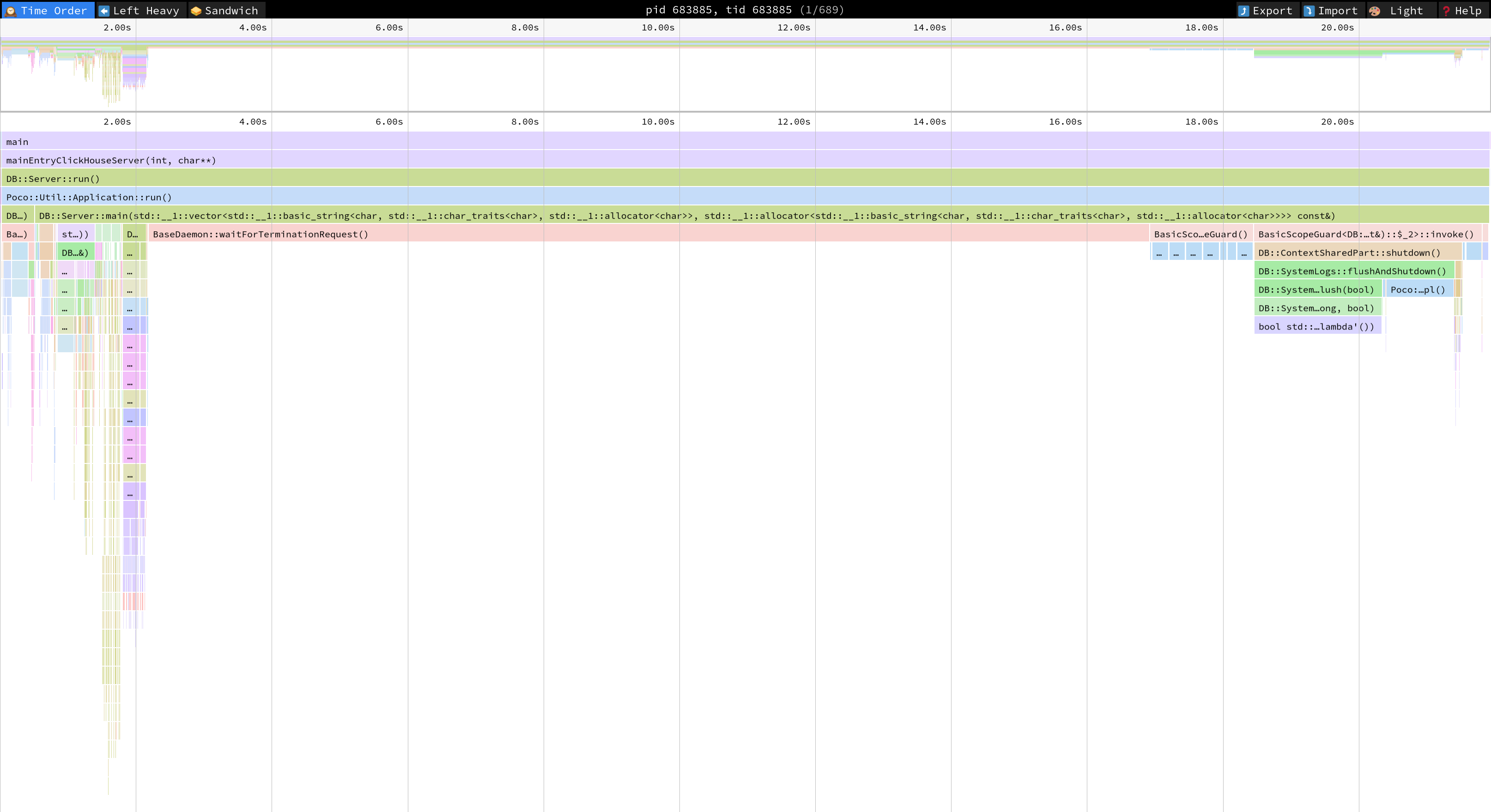
Profiling ClickHouse

  1. Pass -DENABLE_XRAY=1 to cmake when building ClickHouse. This sets the proper compiler flags.
  2. Set XRAY_OPTIONS="patch_premain=true xray_mode=xray-basic verbosity=1 env var when running ClickHouse to generate the trace.
  3. Convert the trace to an interesting format such as trace event: llvm-xray convert --symbolize --instr_map=./build/programs/clickhouse --output-format=trace_event xray-log.clickhouse.ZqKprE | gzip > clickhouse-trace.txt.gz.
  4. Visualize the trace in speedscope.app or Perfetto.

clickhouse-time-order

Notice that this is the visualization of only one thread. You can select the others tids on the top bar.

Check out the docs

Take a look at the XRay Instrumentation and Debugging with XRay documentation to learn more details.

· 4 min read

With the introduction of the new JSON data type, ClickHouse is now a good choice of database for doing JSON analytics. In this guide, we're going to learn how to load JSON messages from Apache Kafka directly into a single JSON column in ClickHouse.

Setup Kafka

Let's start by running a Kafka broker on our machine. We're also going to map port 9092 to port 9092 on our host operating system so that it's easier to interact with Kafka:

docker run --name broker -p 9092:9092 apache/kafka:3.8.1

Ingest data into Kafka

Once that's running, we need to ingest some data. The Wikimedia recent changes feed is a good source of streaming data, so let's ingest that into the wiki_events topic:

curl -N https://stream.wikimedia.org/v2/stream/recentchange 2>/dev/null |
awk '/^data: /{gsub(/^data: /, ""); print}' |
jq -cr --arg sep ø '[.meta.id, tostring] | join($sep)' |
kcat -P -b localhost:9092 -t wiki_events -Kø

We can check tha the data's being ingested by running the following command:

kcat -C -b localhost:9092  -t wiki_events
{"$schema":"/mediawiki/recentchange/1.0.0","meta":{"uri":"https://www.wikidata.org/wiki/Q130972321","request_id":"5c687ded-4721-4bfc-ae6c-58ca25f4a6ce","id":"0fbb0982-c43b-4e8b-989b-db7e78dbdc76","dt":"2024-11-06T11:59:57Z","domain":"www.wikidata.org","stream":"mediawiki.recentchange","topic":"codfw.mediawiki.recentchange","partition":0,"offset":1228777205},"id":2338656448,"type":"edit","namespace":0,"title":"Q130972321","title_url":"https://www.wikidata.org/wiki/Q130972321","comment":"/* wbsetclaim-create:2||1 */ [[Property:P18]]: Mahdi Rrezaei Journalist.jpg","timestamp":1730894397,"user":"Wikimellatir","bot":false,"notify_url":"https://www.wikidata.org/w/index.php?diff=2270885254&oldid=2270870214&rcid=2338656448","minor":false,"patrolled":false,"length":{"old":4269,"new":4636},"revision":{"old":2270870214,"new":2270885254},"server_url":"https://www.wikidata.org","server_name":"www.wikidata.org","server_script_path":"/w","wiki":"wikidatawiki","parsedcomment":"<span dir=\"auto\"><span class=\"autocomment\">Created claim: </span></span> <a href=\"/wiki/Property:P18\" title=\"image | image of relevant illustration of the subject; if available, also use more specific properties (sample: coat of arms image, locator map, flag image, signature image, logo image, collage image)\"><span class=\"wb-itemlink\"><span class=\"wb-itemlink-label\" lang=\"en\" dir=\"ltr\">image</span> <span class=\"wb-itemlink-id\">(P18)</span></span></a>: Mahdi Rrezaei Journalist.jpg"}
{"$schema":"/mediawiki/recentchange/1.0.0","meta":{"uri":"https://www.wikidata.org/wiki/Q75756596","request_id":"eb116219-7372-4725-986f-790211708d36","id":"9e0d5299-5bd1-4c58-b796-9852afd8a84e","dt":"2024-11-06T11:59:54Z","domain":"www.wikidata.org","stream":"mediawiki.recentchange","topic":"codfw.mediawiki.recentchange","partition":0,"offset":1228777206},"id":2338656449,"type":"edit","namespace":0,"title":"Q75756596","title_url":"https://www.wikidata.org/wiki/Q75756596","comment":"/* wbeditentity-update-languages-and-other:0||55 */ mv labels and aliases matching [[Property:P528]] or [[Property:P3083]] to mul","timestamp":1730894394,"user":"Twofivesixbot","bot":true,"notify_url":"https://www.wikidata.org/w/index.php?diff=2270885237&oldid=2147709089&rcid=2338656449","minor":false,"patrolled":true,"length":{"old":30879,"new":27161},"revision":{"old":2147709089,"new":2270885237},"server_url":"https://www.wikidata.org","server_name":"www.wikidata.org","server_script_path":"/w","wiki":"wikidatawiki","parsedcomment":"<span dir=\"auto\"><span class=\"autocomment\">Changed label, description and/or aliases in 55 languages, and other parts: </span></span> mv labels and aliases matching <a href=\"/wiki/Property:P528\" title=\"catalog code | catalog name of an object, use with qualifier P972\"><span class=\"wb-itemlink\"><span class=\"wb-itemlink-label\" lang=\"en\" dir=\"ltr\">catalog code</span> <span class=\"wb-itemlink-id\">(P528)</span></span></a> or <a href=\"/wiki/Property:P3083\" title=\"SIMBAD ID | identifier for an astronomical object, in the University of Strasbourg&#039;s SIMBAD database\"><span class=\"wb-itemlink\"><span class=\"wb-itemlink-label\" lang=\"en\" dir=\"ltr\">SIMBAD ID</span> <span class=\"wb-itemlink-id\">(P3083)</span></span></a> to mul"}

So far, so good.

Ingest data into ClickHouse

Next, we're going to ingest the data into ClickHouse. First, let's enable the JSON type (which is currently experimental), by setting the following property:

SET allow_experimental_json_type = 1;

Now, we'll create the wiki_queue table, which uses the Kafka table engine.

CREATE TABLE wiki_queue
(
json JSON
)
ENGINE = Kafka(
'localhost:9092',
'wiki_events',
'clickhouse-consumer-group',
'JSONAsObject'
);

Note that we're using the JSONAsObject format, which will ensure that incoming messages are made available as a JSON object. This format can only be parsed into a table that has a single column with the JSON type.

Next, we'll create the underlying table to store the Wiki data:

CREATE TABLE wiki
(
json JSON,
id String MATERIALIZED getSubcolumn(json, 'meta.id')
)
ENGINE = MergeTree
ORDER BY id;

Finally, let's create a materialized view to populate the wiki table:

CREATE MATERIALIZED VIEW wiki_mv TO wiki AS 
SELECT json
FROM wiki_queue;

Querying JSON data in ClickHouse

We can then write queries against the wiki table. For example, we could count the number of bots that have committed changes:

SELECT json.bot, count()
FROM wiki
GROUP BY ALL
   ┌─json.bot─┬─count()─┐
1. │ true │ 2526 │
2. │ false │ 4691 │
└──────────┴─────────┘

Or we could find out the users that make the most changes on en.wikipedia.org:

SELECT
json.user,
count()
FROM wiki
WHERE json.server_name = 'en.wikipedia.org'
GROUP BY ALL
ORDER BY count() DESC
LIMIT 10
    ┌─json.user──────────────────────────────┬─count()─┐
1. │ Monkbot │ 267 │
2. │ Onel5969 │ 107 │
3. │ Bangwiki │ 37 │
4. │ HHH Pedrigree │ 28 │
5. │ REDACTED403 │ 23 │
6. │ KylieTastic │ 22 │
7. │ Tinniesbison │ 21 │
8. │ XTheBedrockX │ 20 │
9. │ 2001:4455:1DB:4000:51F3:6A16:408E:69FC │ 19 │
10. │ Wcquidditch │ 15 │
└────────────────────────────────────────┴─────────┘

· 2 min read

Question

How can I connect to ClickHouse using SSH Key Authentication?

Note

We use ClickHouse Cloud as an example here, but this example should also work on oss ClickHouse.

Answer

1) Use ssh-keygen to create the keypair. Example:

➜  new ssh-keygen \
-t ed25519 \
> -f /Users/testuser/.ssh/ch_key
Generating public/private ed25519 key pair.
Enter passphrase (empty for no passphrase):
Enter same passphrase again:
Your identification has been saved in /Users/testuser/.ssh/ch_key
Your public key has been saved in /Users/testuser/.ssh/ch_key.pub
.....

2) Use the public key (ch_key.pub in above example) to create the USER.

clickhouse-cloud :) CREATE USER abcuser IDENTIFIED WITH ssh_key BY KEY 'AAAABBBcdE1lZDI1NTE5AAAAIISdl4CrGM8mckXBUXLjL3ef9XwnycDWEvBPu3toB40m' TYPE 'ssh-ed25519';

CREATE USER abcuser IDENTIFIED WITH ssh_key BY KEY AAAABBBcdE1lZDI1NTE5AAAAIISdl4CrGM8mckXBUXLjL3ef9XwnycDWEvBPu3toB40m TYPE `ssh-ed25519`

Query id: 34c6aad6-5f88-4c80-af7a-7d37c91ba7d5

Ok.

3) Run SHOW users to confirm the user creation.

4) Grant default_role to the user (optional).

clickhouse-cloud :) grant default_role to abcuser;

GRANT default_role TO abcuser

Query id: 4a054003-220a-4dea-8e8d-eb1f08ee7b10

Ok.

0 rows in set. Elapsed: 0.137 sec.

5) Use the private key now to authenticate against the service.

➜  new ./clickhouse client --host myhost.us-central1.gcp.clickhouse.cloud --secure --user abcuser --ssh-key-file '/Users/testuser/.ssh/ch_key'
ClickHouse client version 23.12.1.863 (official build).
Enter your private key passphrase (leave empty for no passphrase):
Connecting to myhost.us-central1.gcp.clickhouse.cloud:9440 as user abcuser.
Connected to ClickHouse server version 23.9.2.

clickhouse-cloud :) select currentUser();

SELECT currentUser()

Query id: d4b6bb60-ef45-47d3-8740-db9f2941dcd2

┌─currentUser()─┐
│ abcuser │
└───────────────┘

1 row in set. Elapsed: 0.001 sec.

clickhouse-cloud :)

· 3 min read

The table below provides the mapping for the metrics used in system.dashboards to Prometheus metrics in system.custom_metrics.
This is useful for customers who want to monitor for the same metrics found in system.dashboards.

Mapping table for metrics in system.dashboards to Prometheus metrics in system.custom_metrics

DashboardTitlePrometheus Metric Name (system.custom_metrics)
OverviewQueries/secondClickHouseProfileEvents_Query
OverviewCPU Usage (cores)ClickHouseProfileEvents_OSCPUVirtualTimeMicroseconds
OverviewQueries RunningClickHouseMetrics_Query
OverviewMerges RunningClickHouseMetrics_Merge
OverviewSelected Bytes/secondClickHouseProfileEvents_SelectedBytes
OverviewIO WaitClickHouseProfileEvents_OSIOWaitMicroseconds
OverviewCPU WaitClickHouseProfileEvents_OSCPUWaitMicroseconds
OverviewOS CPU Usage (Userspace)ClickHouseAsyncMetrics_OSUserTimeNormalized
OverviewOS CPU Usage (Kernel)ClickHouseAsyncMetrics_OSSystemTimeNormalized
OverviewRead From DiskClickHouseProfileEvents_OSReadBytes
OverviewRead From FilesystemClickHouseProfileEvents_OSReadChars
OverviewMemory (tracked)ClickHouseMetrics_MemoryTracking
OverviewLoad Average (15 minutes)ClickHouseAsyncMetrics_LoadAverage15
OverviewSelected Rows/secondClickHouseProfileEvents_SelectedRows
OverviewInserted Rows/secondClickHouseProfileEvents_InsertedRows
OverviewTotal MergeTree PartsClickHouseAsyncMetrics_TotalPartsOfMergeTreeTables
OverviewMax Parts For PartitionClickHouseAsyncMetrics_MaxPartCountForPartition
Cloud overviewQueries/secondClickHouseProfileEvents_Query
Cloud overviewCPU Usage (cores)ClickHouseProfileEvents_OSCPUVirtualTimeMicroseconds
Cloud overviewQueries RunningClickHouseMetrics_Query
Cloud overviewMerges RunningClickHouseMetrics_Merge
Cloud overviewSelected Bytes/secondClickHouseProfileEvents_SelectedBytes
Cloud overviewIO Wait (local fs)ClickHouseProfileEvents_OSIOWaitMicroseconds
Cloud overviewS3 read waitClickHouseProfileEvents_ReadBufferFromS3Microseconds
Cloud overviewS3 read errors/secProfileEvent_ReadBufferFromS3RequestsErrors
Cloud overviewCPU WaitClickHouseProfileEvents_OSCPUWaitMicroseconds
Cloud overviewOS CPU Usage (Userspace, normalized)ClickHouseAsyncMetrics_OSUserTimeNormalized
Cloud overviewOS CPU Usage (Kernel, normalized)ClickHouseAsyncMetrics_OSSystemTimeNormalized
Cloud overviewRead From Disk (bytes/sec)ClickHouseProfileEvents_OSReadBytes
Cloud overviewRead From Filesystem (bytes/sec)ClickHouseProfileEvents_OSReadChars
Cloud overviewMemory (tracked, bytes)ClickHouseMetrics_MemoryTracking
Cloud overviewLoad Average (15 minutes)ClickHouseAsyncMetrics_LoadAverage15
Cloud overviewSelected Rows/secClickHouseProfileEvents_SelectedRows
Cloud overviewInserted Rows/secClickHouseProfileEvents_InsertedRows
Cloud overviewTotal MergeTree PartsClickHouseAsyncMetrics_TotalPartsOfMergeTreeTables
Cloud overviewMax Parts For PartitionClickHouseAsyncMetrics_MaxPartCountForPartition
Cloud overviewRead From S3 (bytes/sec)ClickHouseProfileEvents_ReadBufferFromS3Bytes
Cloud overviewFilesystem Cache SizeClickHouseMetrics_FilesystemCacheSize
Cloud overviewDisk S3 write req/secClickHouseProfileEvents_DiskS3PutObject + ClickHouseProfileEvents_DiskS3UploadPart + ClickHouseProfileEvents_DiskS3CreateMultipartUpload + ClickHouseProfileEvents_DiskS3CompleteMultipartUpload
Cloud overviewDisk S3 read req/secClickHouseProfileEvents_DiskS3GetObject + ClickHouseProfileEvents_DiskS3HeadObject + ClickHouseProfileEvents_DiskS3ListObjects
Cloud overviewFS cache hit rateClickHouseProfileEvents_CachedReadBufferReadFromCacheBytes / (ClickHouseProfileEvents_CachedReadBufferReadFromCacheBytes + ClickHouseProfileEvents_CachedReadBufferReadFromSourceBytes)
Cloud overviewPage cache hit rategreatest(0, (sum(ClickHouseProfileEvents_OSReadChars) - sum(ClickHouseProfileEvents_OSReadBytes)) / (sum(ClickHouseProfileEvents_OSReadChars) + sum(ClickHouseProfileEvents_ReadBufferFromS3Bytes)))
Cloud overviewNetwork receive bytes/secClickHouseProfileEvents_NetworkReceiveBytes
Cloud overviewNetwork send bytes/secClickHouseProfileEvents_NetworkSendBytes

Related links:
https://clickhouse.com/docs/en/integrations/prometheus

· One min read

Question

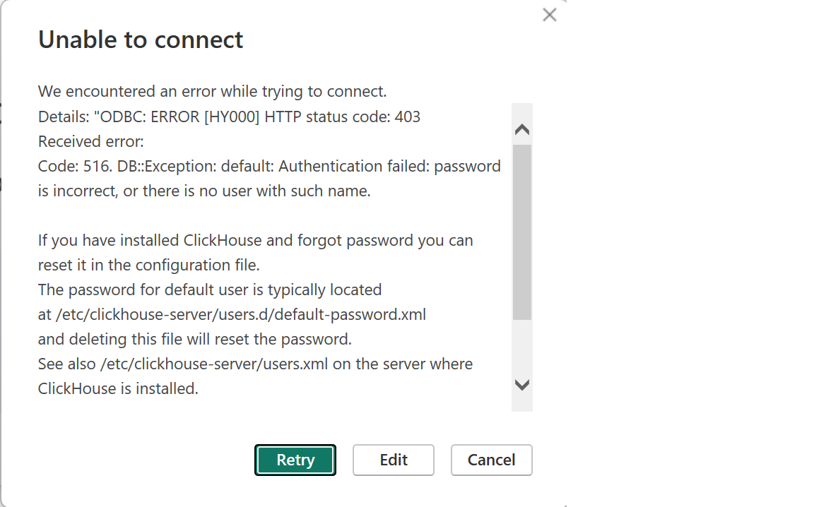
When trying to connect from PowerBI to ClickHouse using the connector, you receive the following authentication error:

We encountered an error while trying to connect.
Details: "ODBC: ERROR [HY000] HTTP status code: 403
Received error:
Code: 516. DB::Exception: default: Authentication failed: password is incorrect, or there is no user with such name.
If you have installed ClickHouse and forgot password you can reset it in the configuration file.
The password for default user is typically located at /etc/clickhouse-server/users.d/default-password.xml and deleting this file will reset the password.
See also /etc/clickhouse-server/users.ml on the server where
ClickHouse is installed.

powerbi_error

Answer

Check the password being used to see if the password contains a tilde ~.

The recommendation is to use a dedicated user for the connection and set the password manually. If using ClickHouse Cloud and the admin level of permissions with the default user is needed, then create a new user and and assign the default_role.

For more information:
https://clickhouse.com/docs/en/operations/access-rights#user-account-management
https://clickhouse.com/docs/en/cloud/security/cloud-access-management#database-roles

· 2 min read

Question

How do I create a table that can query other clusters or instances?

Answer

Below is a simple example to test functionality.

In this example, ClickHouse Cloud is use but the example will work when using self-hosted clusters also. The targets will need to change to the urls/hosts/dns of a target node or load balancer.

In cluster A:

./clickhouse client --host clusterA.us-west-2.aws.clickhouse.cloud --secure --password 'Password123!'

Create the database:

create database db1;

Create the table:

 CREATE TABLE db1.table1_remote1
(
`id` UInt32,
`timestamp_column` DateTime,
`string_column` String
)
ENGINE = MergeTree()
ORDER BY id;

Insert some sample rows:

insert into db1.table1_remote1
values
(1, '2023-09-29 00:01:00', 'a'),
(2, '2023-09-29 00:02:00', 'b'),
(3, '2023-09-29 00:03:00', 'c');

In cluster B:

./clickhouse client --host clusterB.us-east-2.aws.clickhouse.cloud --secure --password 'Password123!'

Create the database:

create database db1;

Create the table:

CREATE TABLE db1.table1_remote2
(
`id` UInt32,
`timestamp_column` DateTime,
`string_column` String
)
ENGINE = MergeTree()
ORDER BY id;

Insert sample rows:

insert into db1.table1_remote1
values
(4, '2023-09-29 00:04:00', 'x'),
(5, '2023-09-29 00:05:00', 'y'),
(6, '2023-09-29 00:06:00', 'z');

In Cluster C:
*this cluster will be used to gather the data from the other two clusters, however, can also be used as a source.

./clickhouse client --host clusterC.us-west-2.aws.clickhouse.cloud --secure --password 'Password123!'

Create the database:

create database db1;

Create the remote tables with remoteSecure() to connect to the other clusters.
Definition for remote cluster A table:

CREATE TABLE db1.table1_remote1_main
(
`id` UInt32,
`timestamp_column` DateTime,
`string_column` String
) AS remoteSecure('clusterA.us-west-2.aws.clickhouse.cloud:9440', 'db1.table1_remote1', 'default', 'Password123!');

Definition for remote cluster B table:

CREATE TABLE db1.table1_remote2_main
(
`id` UInt32,
`timestamp_column` DateTime,
`string_column` String
) AS remoteSecure('clusterB.us-east-2.aws.clickhouse.cloud:9440', 'db1.table1_remote2', 'default', 'Password123!')

Create the merge table to be used to gather results:

create table db1.table1_merge_remote
(
id UInt32,
timestamp_column DateTime,
string_column String
)
engine = Merge('db1', 'table.\_main');

Test the results:

clickhouse-cloud :) select * from db1.table1_merge_remote;

SELECT *
FROM db1.table1_merge_remote

Query id: 46b6e741-bbd1-47ed-b40e-69ddb6e0c364

┌─id─┬────timestamp_column─┬─string_column─┐
│ 1 │ 2023-09-29 00:01:00 │ a │
│ 2 │ 2023-09-29 00:02:00 │ b │
│ 3 │ 2023-09-29 00:03:00 │ c │
└────┴─────────────────────┴───────────────┘
┌─id─┬────timestamp_column─┬─string_column─┐
│ 4 │ 2023-09-29 00:04:00 │ x │
│ 5 │ 2023-09-29 00:05:00 │ y │
│ 6 │ 2023-09-29 00:06:00 │ z │
└────┴─────────────────────┴───────────────┘

6 rows in set. Elapsed: 0.275 sec.

For more info:
https://clickhouse.com/docs/en/sql-reference/table-functions/remote
https://clickhouse.com/docs/en/engines/table-engines/special/merge

· 4 min read

Question

What data types should I use in ClickHouse to optimize my queries for speed and storage?

Answer

Many times when using an automated conversion from another system or trying to choose a data type, users will often choose the "more is better" or "choose what's easier" or "choose the most generic" approaches. This will likely work for small datasets in the millions, maybe even billions of rows. It may not be noticeable and is acceptable for those type of sets where users' queries difference is small in their use-cases.

It will not be acceptable, however, as the data grows and becomes more noticeable.

The difference between a query taking 50ms and 500ms may be okay for most use-cases, for example in a webUI, but one is 10x slower than the other, even though for a front-end user, is not very noticeable.

Example initial table:

timestamp Datetime64(9),
group_id Int64,
vendor_id String,
product_id String,
category1 Int64,
code_name String,
paid_status String,
country_code String,
description String,
price Float64,
attributes Map(String, String)

Sample data:

3456, 0123456789, bd6087b7-6026-4974-9122-bc99faae5d84, "2024-03-01 01:00:01.000", 98, "bear", paid", "us", "corvette model car", 123.45, {"color" : "blue", "size" : "S"}
156, 0000012345, bd6087b7-6026-4974-9122-bc99faae5d84, "2024-03-01 01:00:02:123", 45, "tiger", "not paid", "uk", "electric car", 53432.10, {"color" : "red", "model" : "X"}
...

Below are some recommendations where this data could be optimized:

timestamp : DateTime64(9)
Unless needing scientific precision, a value of 9 precision (nanoseconds), is unlikely necessary. Possibly could be for display or ordering, but usually not in queries for searching, primary keys, etc.

  • Recommendation:
    For PK, order by: DateTime
    For display or ordering: add additional column - i.e. timestamp_microseconds : DateTime64(6)

group_id : Int64
This appears to be an integer, select the smallest integer type that will fit the max number for the column required. From this sample dataset and name of the column, it is unlikely to need a quintillion values, probably an Int16 would work where it could have up to 16k values.

  • Recommendation: Int16

vendor_id : String
This column looks like to be a number but has leading zeros, likely important to keep formatting. Also appears to be only a certain number of chars.

  • Recommendation: FixedString(10)

product_id : String
This one is alphanumeric so intuitively would be a string, however, it is also a UUID.

  • Recommendation: UUID

category1 : Int64
The values are small, probably not very many categories and not looking to grow very much or limited. Less than 255

  • Recommendation: UInt8

code_name : String
This field looks like it may have only a limited number of strings that would be used. For this kind of situation where the number of string values might be in the hundreds or thousands, low cardinality fields help.

  • Recommendation: LowCardinality(String)

paid_status : String
There is a string value of "paid" or "not_paid". For situations where there may be only two values, use a boolean.

  • Recommendation: Bool

country_code : String
Sometimes there are columns which meet multiple optimizations. In this example, there are only a certain number of country codes and they are all two character identifiers.

  • Recommendation: LowCardinality(FixedString(2))

price : Float64
Floats are not recommended when there is a fixed precision that is known, especially for financial data and calculations. Best is to use Decimal types for the precision necessary. For this use-case, it is likely that the price of the item is not over 999,999.00

  • Recommendation: Decimal(10,2)

attributes : map
Often there might be a table with dynamic attributes in maps. Searching for keys or values is usually slower. There’s a couple of ways that the maps can be made faster. If there are keys that will be present in most records, best to place those in a separate column as low cardinality and those that will be sparse in another column high cardinality. From there, it will be more efficient to create skip indexes although it may increase the complexity of the queries.

  • Recommendation: lc_attributes: Map(String, String), hc_attributes: Map(String, String).

Depending on the queries, the options that can also be used to create a skip index and/or extract the attributes are:
Using Array Join to extract into columns using a Materialized View: https://clickhouse.com/docs/knowledgebase/using-array-join-to-extract-and-query-attributes
Using a skip index for the keys: https://clickhouse.com/docs/knowledgebase/improve-map-performance